By substituting the Hertzian contact parameters (in terms of the applied load and contact geometry), they obtained the load-life relationship for rolling bearings. This can be expressed in its final form in a very simple way:

SKFbearing life calculationpdf

Responder: Ângulo correspondente a C: 130∘130^{\circ}130∘, Ângulo correspondente a A: 250∘250^{\circ}250∘, Ângulo correspondente a B: 340∘340^{\circ}340∘.

Ballbearing lifein hours

Select your vehicle ; Raybestos Wheel Bearing And Hub Assembly. $30.00 – $354.00 ; Wilwood Front Hub Kit. $625.00 ; Quality-Built Wheel Hubs and Bearings. $17.00 – ...

35TGV470M12.5X13.5 Rubycon Aluminum Electrolytic Capacitors - SMD HIGH TEMPERATURE ELECTROLYTIC CAPACITORS datasheet, inventory, & pricing.

The demands for safe design and lighter, competitively priced products have put a new emphasis on predictability of rolling bearing performance. This has prompted researchers to update standards for bearing life to take into account progress in engineering technology.

ii) consideration of the stressed volume below a contact as an array of relatively small volume elements, each experiencing individual local stresses.

This is the formulation of the life equation used in the SKF General Catalogue since 1989. This equation, in conjunction with the diagrams of figures 1 and 2, can be used to calculate the life of rolling bearings in a straightforward manner that is similar to the previous life calculation, ISO 281:1990. However, equation 10 can account for specific lubrication and contamination conditions of the bearing and for the increased life that is experienced in case of lightly loaded, clean and well lubricated bearing applications.

Bearing life calculationformula

where the h parameter is a factor (corresponding to a stress factor) that is introduced to account for the actual stresses present in real bearing contacts. This parameter is not included with the ideal Hertzian stress field used in the derivation of the original Lundberg and Palmgren (1947) life formula. It can be shown that, besides the bulk stresses due to the heat treatment and mounting, the stress factor h depends to a large extent on the lubrication condition of the contact and on micro-scale stress concentrations due to denting or imperfections. Consequently, h is given as a function of the environmental conditions, (lubrication and contamination), and in relation to the bearing size.

Present standards for bearing life calculation are based on work carried out at SKF in 1947 by Gustaf Lundberg and Arvid Palmgren. The life equation was formulated using the Weibull probability theory of fatigue developed in 1936. This allowed the calculation to include bearing reliability. It marked a substantial step forward in the achievement of predictive methods for the applications of this essential machine element. The ability to estimate the life of a bearing and to select, on a rational basis, a specific bearing suitable for a particular application was a breakthrough for engineering design. Since then, science and technology, in particular tribology, have made tremendous strides. The latest theoretical knowledge and calculation techniques supported by powerful modern computers are now applied in bearing technology and design work. Also, steel manufacturers can make cleaner steels to more accurate and consistent formulations. In addition, greatly improved lubricants allow better separation than before of moving contacting surfaces in rolling bearings, while modern mass production manufacturing methods produce high precision bearings to ever-higher levels of quality. Such technological progress requires that bearing life calculations take into account the improved performance of today’s bearings. Over the years, performance improvements were accounted for largely through increased dynamic load ratings, which yielded longer calculated lives. Application or adjustment factors were sometimes used to account for operational conditions, such as special bearing materials and lubricants. Until recently, these life calculations served industry sufficiently well. However, observations about the predominant failure mechanisms in modern rolling bearings have added new knowledge in this field. It has been found that fatigue failures are more frequently initiated at the surface rather than from cracks formed beneath the surface. Consequently, attention has been paid to the influence of surface finish and contamination on bearing performance. The existence of a fatigue limit for modern bearing steels has also been observed. Such considerations have resulted in the publication of improved bearing life calculations and papers studying the effects of contamination and surface finish on bearing life.

where C is the bearing basic dynamic load rating, a factor that depends on the bearing geometry, and P is the equivalent bearing load. The exponent p is 3 for ball bearings and 10/3 for roller bearings. Equation 2 was adopted by ISO in the recommendation R281-(1962). In 1977, the multiplicative constants a1, a2 and a3 were introduced to account for different levels of reliability, material fatigue properties and lubrication, resulting in the standard used today, ISO 281 (1990):

SKFbearing lifeCalculator

Furthermore curves of the function hc(k,dm, bcc) were also derived, as explained by Bergling and Ioannides (1994) and Ioannides and his colleagues (1999). Examples of these parametric curves are given in figure 2. With this information, the life equation 8 can be written in a simple way:

SKF ballbearing life calculation

We would like to find out what you think about SKF Evolution, so that it can be improved. We would really appreciate you helping us by answering a few questions. Many thanks!

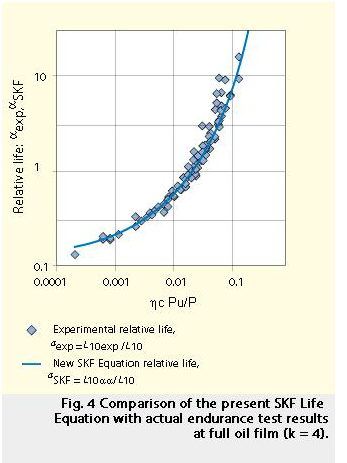
Experimental verification To verify the accuracy of the SKF Bearing Life Equation (equation 10), extensive bearing endurance tests were performed on more than 8,000 bearings under a variety of lubrication and contamination test conditions. An overview of the mean L10 measured in these tests is shown in figure 3. A comparison was made between predicted lives and the actual endurance test data of figure 3. This was performed by plotting the ratio between the experimental bearing life and the basic rating life of the bearing, i.e. aexp=L10exp/ L10 versus the corresponding stress factor parameter, hcPu/P. In figure 4, a group of experimental points of ball bearing operating with a full oil film is shown. The data points of the test results mostly overlap with the corresponding life-ratio curve, i.e. aSKF , calculated according to equation 9. Figure 4 shows very good agreement between the relative life calculated with the SKF Life Equation and the endurance test results. A more comprehensive evaluation of the experimental data also indicated that the total bias in life calculation could be reduced by half using the SKF Life Equation in comparison to the results of life calculations based only on bearing standard ratings. This improved accuracy provides a better match between theory and test data, validating the choice of the model constants used and the present Life Equation. Furthermore, the asymptotic trend displayed by the function aSKF (k, hc Pu/P), figures 1 and 4 as the stress factor parameter hc Pu/Ptends towards lower stress conditions for the bearing, and is a further indication of the postulated fatigue stress limit in rolling contact fatigue. The behaviour of the curve aSKF(relative stress vs. relative life) is indeed similar to the familiar Wöhler (stress vs. number of stress cycles) curves used for plotting the survival probability of specimens subjected to fatigue testing at different stress level.

Conclusions Rolling bearings have made it possible to support heavy loads at high rotational speeds with good reliability and a minimum of friction. This basic technology has allowed the massive mechanisation process that has characterised the past century and has profoundly revolutionised our way of life. Practical tools for better selection and use of rolling bearings have a significant effect on the way machines operate, their efficiency and cost. This affects each of us through the energy consumption and running costs of society at large. The SKF Life Equation introduces a new and higher standard in life calculations to help in the prediction of bearing performance and to respond to the continual quest for better ways to design, select and use bearings. The SKF Life Equation manages to describe the complex tribo-system in which the bearing operates using a few key parameters. This is an important feature of the model that concentrates on the effect of a few important factors that have significant consequences for the bearing life. Furthermore, the SKF Life Equation recognises that the fatigue effect arising from these factors cannot be written as a linear superposition of the risks induced from individual stress components. Rather than attempting to derive independent life modifying factors for lubrication, contamination etc., a single multidimensional factor, aSKF = f (k, hc Pu/P), is introduced depending on those relevant factors describing the tribo-physical state of the system. By this approach, the best use is made of the available input data, to the benefit of both the designer and the user of a machine. The good agreement with the experimental results and improved accuracy achieved using the SKF Life Equation support the use of this approach for the calculation of the life expectancy of modern rolling bearings.

Ioannides E., Bergling G. and Gabelli A. “An analytical formulation for the life of rolling bearings.” Acta Polytechnica Scandinavica, ME 137, Espoo (1999).

Bearing life calculationexcel

In this way, real local stresses and many effects stemming from surface stress concentrations, such as edge stresses and contamination dents, can be introduced consistently into fatigue life predictions. Such a comprehensive approach requires access to complex computer programs for bearing life calculations, as integration of the failure risk over complicated stress fields is required. Many bearing users do not have access to such resources. Instead they usually apply simple formulae readily available in bearing manufacturers’ catalogues or standards. To support these needs, and reap the benefits provided by advances in technology and knowledge, the SKF Life Equation was made available. This equation was developed by introducing an effective real weighted stress that is averaged throughout the risk volume. The fatigue limit and the local stress were implemented into equations similar to those used by Lundberg-Palmgren. In practice, this is done by introducing a stress factor that acts on the fatigue limit of the bearing. This factor accounts for the actual stress condition of real bearings but is not included with the ideal Hertzian stress field, as used in the Lundberg-Palmgren classical analysis. This approach led to a simple expression that can be readily calculated in a similar way to the ISO 281 (1990) formulation. This equation retains much of the original simplicity of the load-life equation but also describes the performance of modern bearings more accurately than before.

Replacement Steering Column Upper Bearing Kit for Ford F-450 Super Duty OE F4DZ-3517-A, Wear Corrosion Resistant

Hex 802020 color converted to 17 different formats like RGB, CMYK, HSV, HSL.The Hex color 802020 is a dark color, and the websafe version is hex 993333.

Mounting holes are prepared on outer ring and inner ring providing easy mounting together with high rigidity and high accuracy. Table 1 Crossed Roller Bearing ...

Ballbearing lifecalculator

In particular, the rolling contact fatigue life model published by Eustathios Ioannides and Tedric Harris (1985) introduced two innovations to the Lundgren and Palmgren theory:

To simplify the use of the above equation, in 1989 SKF introduced a Stress Life Factor aSKF for each specific bearing (brg) class: radial ball bearings, radial roller bearings, thrust ball bearings, thrust roller bearings. This factor can be calculated and plotted as shown in figure 1:

202337 — Save time & hassle with the Speedi-Bleed pressure brake bleeder. Firmer pedal & cleaner fluid. Discover just how easy bleeding brakes can be.

In the above formulation, Macauley bracket notation is used; in other words, the term is set to zero if the quantity enclosed is negative. To obtain the Life Equation for rolling bearings in the presence of a material fatigue limit, one may use equation 5. This equation differs from the original Lundberg and Palmgren form (equation 1) only by the Macauley bracket on the right side of equation 5. It is, therefore, possible to work through the bearing capacity formulation very much as in Lundberg and Palmgren’s original work. Applying the well-known relationship between induced stresses and applied load for Hertzian contacts, either point or line, as done by Lundberg and Palmgren (1947), an equation corresponding to equation 5, but written in terms of the equivalent load and the basic dynamic load rating, is obtained. For 10 percent probability of failure, the corresponding bearing life is expressed as :

Ângulo correspondente a C: 130∘130^{\circ}130∘ Ângulo correspondente a A: 250∘250^{\circ}250∘ Ângulo correspondente a B: 340∘340^{\circ}340∘

Eustathios Ioannides, SKF Engineering and Research Centre (ERC), Nieuwegein, the Netherlands & Imperial College of Science, Technology and Medicine, London, UK; Gunnar Bergling, AB SKF, Gothenburg, Sweden, and Antonio Gabelli, SKF Engineering and Research Centre (ERC), Nieuwegein, the Netherlands.

Bearing lifein hours

SKF life formula A simple analytical formulation for bearing life that includes consideration of the fatigue strength of the material evolved from the rolling contact fatigue model set forth by Ioannides and Harris (1985). This was initially applied in the numerical solutions of the fatigue risk of 3-D stress fields of rolling contacts. Due to the self-similarity of Hertzian stress fields, it was found that in the case of strictly Hertzian contacts, simplification was possible. This could be introduced by applying stress criteria based on the maximum alternating shear stress amplitude tO above a threshold value and of a fatigue limit stress tu of the rolling contact . Thus the introduction of the fatigue limit stress tu can be effected through the replacement of the shear stress amplitudetO of the Hertzian stress field of equation 1, by the difference tO – tu . Then equation 1 becomes:

One might think there were no Philistine polities anymore but on this map there are still Philistine city states when the Kingdom of Israel existed.

LINCOLN INDUSTRIAL CORP. · 34089 (PISTON PACKING) · 86233 (REPAIR KIT) · 244883 (QUICKLINC W/CHECK 252751) · 84968 (AIR VALVE KIT) · 84967 (PILOT BAR KIT).

Search the most complete 16143, PA real estate listings for sale. Find 16143, PA homes for sale, real estate, apartments, condos, townhomes, mobile homes, ...

2021820 — We propose to transfer the remainder of the Alemite pump assembly to [our facility] in Johnson City, Tennessee, read the January 31 letter ...

Standardised life equations Fatigue life modelling is central to all bearing life prediction. The traditional crack initiation or cumulative damage model invokes a stress power law to account for the portion of the life spent in the initiation of a crack, which dominates the complete lifetime of rolling contacts. Probabilistic methods were applied early in bearing endurance prediction because of the natural dispersion of bearing life. Lundberg and Palmgren (1947) used the Weibull (1939) probability distribution of metal fatigue to establish the basic theory of the stochastic dispersion of bearing lives, as shown by the equation below:

Want to learn more about what is driving change in the engineering world? EVOLUTION helps you to stay up to date with emerging trends as well as the latest technology. Sign up for EVOLUTION updates to receive new content directly to your inbox.